Palmer Penguins Data Analysis Series (Part 1): Exploratory Data Analysis and Simple Regression

Getting acquainted with our Antarctic friends and their morphometric relationships

Part 1 of a comprehensive 5-part series exploring Palmer penguin morphometrics through exploratory data analysis and simple regression modeling

Curious Adelie penguins beginning their data science journey - because every great analysis starts with getting to know your data!

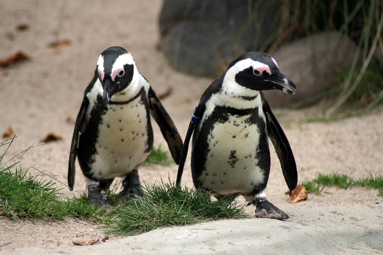
Photo: African penguins at Boulders Beach, South Africa. Licensed under CC BY 2.0 via Wikimedia Commons

Palmer Penguins Data Analysis Series

This is Part 1 of a 5-part series exploring penguin morphometrics:

1. Part 1: EDA and Simple Regression (This post)
2. Part 2: Multiple Regression and Species Effects
3. Part 3: Advanced Models and Cross-Validation
4. Part 4: Model Diagnostics and Interpretation
5. Part 5: Random Forest vs Linear Models

1 Introduction

Welcome to our comprehensive exploration of the Palmer penguins dataset! In this 5-part series, we’ll journey through the complete data science workflow, from initial data exploration to advanced modeling techniques. The Palmer penguins dataset has become a beloved alternative to the iris dataset, providing real-world biological data that’s both engaging and educationally valuable.

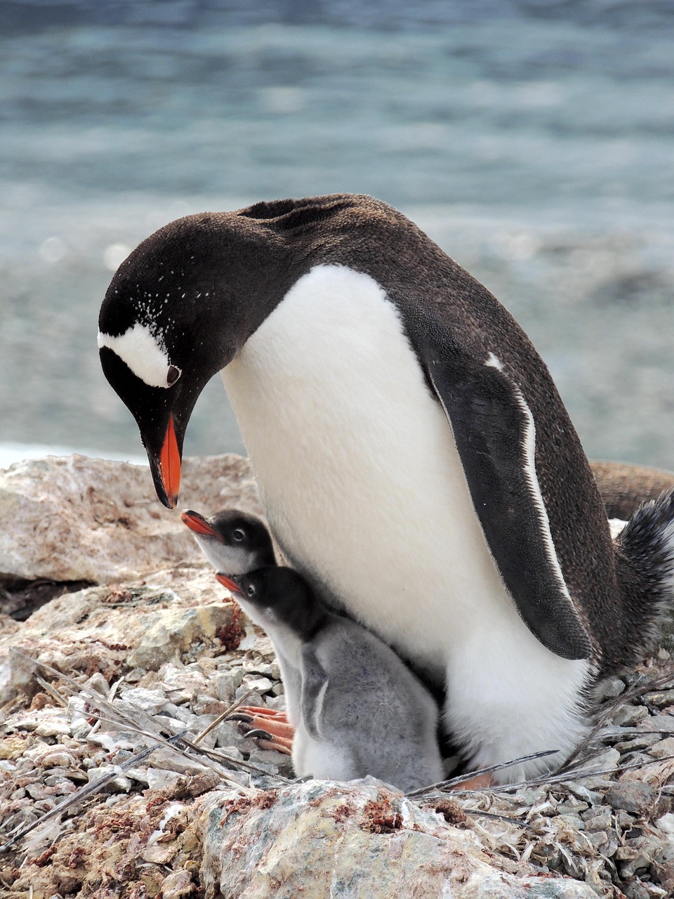
Collected by Dr. Kristen Gorman at Palmer Station Antarctica, this dataset contains morphometric measurements for three penguin species: Adelie (Pygoscelis adeliae), Chinstrap (Pygoscelis antarcticus), and Gentoo (Pygoscelis papua). Understanding these relationships is crucial for Antarctic ecology research, as body mass serves as a key indicator of penguin health and reproductive success.

In this first part, we’ll focus on:

• Getting familiar with the Palmer penguins dataset
• Conducting thorough exploratory data analysis
• Understanding the relationships between morphometric variables
• Building our first simple regression model
• Establishing the foundation for more complex analyses in subsequent parts

By the end of this post, you’ll have a solid understanding of the data structure and the strongest individual predictors of penguin body mass.

2 Prerequisites and Setup

Before we begin our Antarctic adventure, let’s ensure we have the right tools:

Required Packages:

# Install required packages if not already installed
install.packages(c("palmerpenguins", "tidyverse", "broom", "corrplot",
                   "GGally", "patchwork", "knitr"))

Load Libraries:

library(palmerpenguins)
library(tidyverse)
library(broom)
library(corrplot)
library(GGally)
library(patchwork)
library(knitr)

# Set theme for consistent plotting
theme_set(theme_minimal(base_size = 12))

# Set penguin-friendly colors (high contrast)
penguin_colors <- c("Adelie" = "#FF6B6B", "Chinstrap" = "#9B59B6", "Gentoo" = "#2E86AB")

3 Meet the Penguins: Dataset Overview

Let’s start by getting acquainted with our Antarctic research subjects:

Palmer Penguins Dataset Characteristics

Total Observations	333
Variables	9
Species	0
Islands	0
Year Range	2007–2009

Our analysis includes 333 complete penguin observations from three species across three Antarctic islands, spanning the years 2007-2009.

4 Exploratory Data Analysis

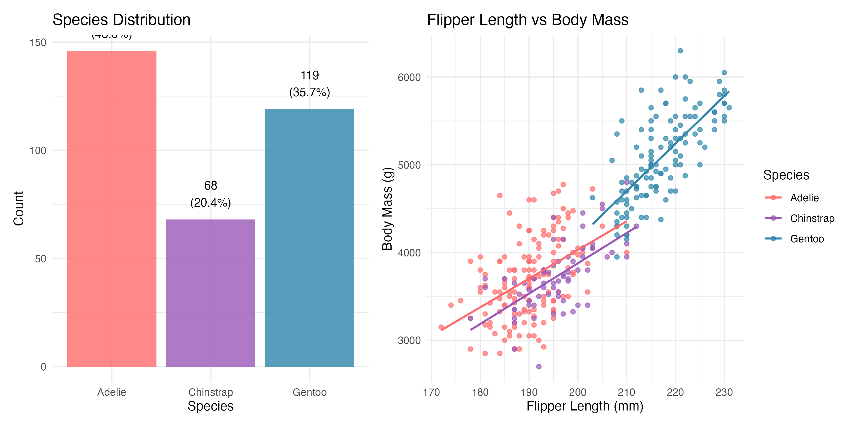
4.1 Species and Morphometric Overview

Let’s understand our penguin community composition and key measurements:

Species Distribution and Key Morphometrics

Species	N	Body Mass (g)	Flipper Length (mm)	% of Dataset
Adelie	146	3706	190.1	43.8
Chinstrap	68	3733	195.8	20.4
Gentoo	119	5092	217.2	35.7

Species distribution and morphometric relationship overview showing sample sizes and the key flipper-body mass relationship across species

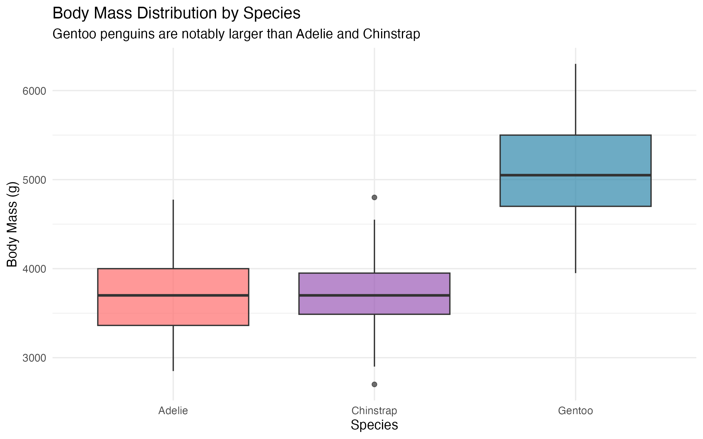
5 Species-Specific Patterns

“Each species has its own personality… and body mass distribution!”

Morphometric Statistics by Species (±95% CI)

Species	N	Body Mass (g)	±95% CI	Flipper Length (mm)	±95% CI
Adelie	146	3706	74.4	190.1	1.1
Chinstrap	68	3733	91.4	195.8	1.7
Gentoo	119	5092	90.1	217.2	1.2

Box plot comparing body mass distributions across the three penguin species, showing Gentoo penguins are substantially larger

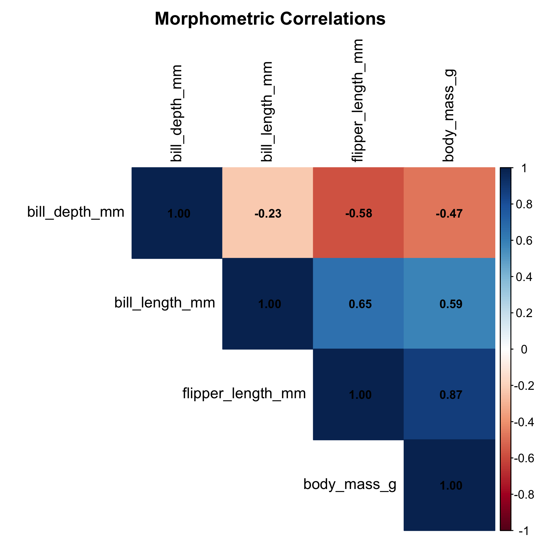
6 Correlation Analysis

Morphometric Correlations with Body Mass

Variable	Correlation with Body Mass	Interpretation
Flipper Length	0.873	Strongest predictor
Bill Length	0.589	Moderate positive
Bill Depth	-0.472	Weak negative

Correlation matrix showing flipper length as the strongest predictor of body mass (r=0.87)

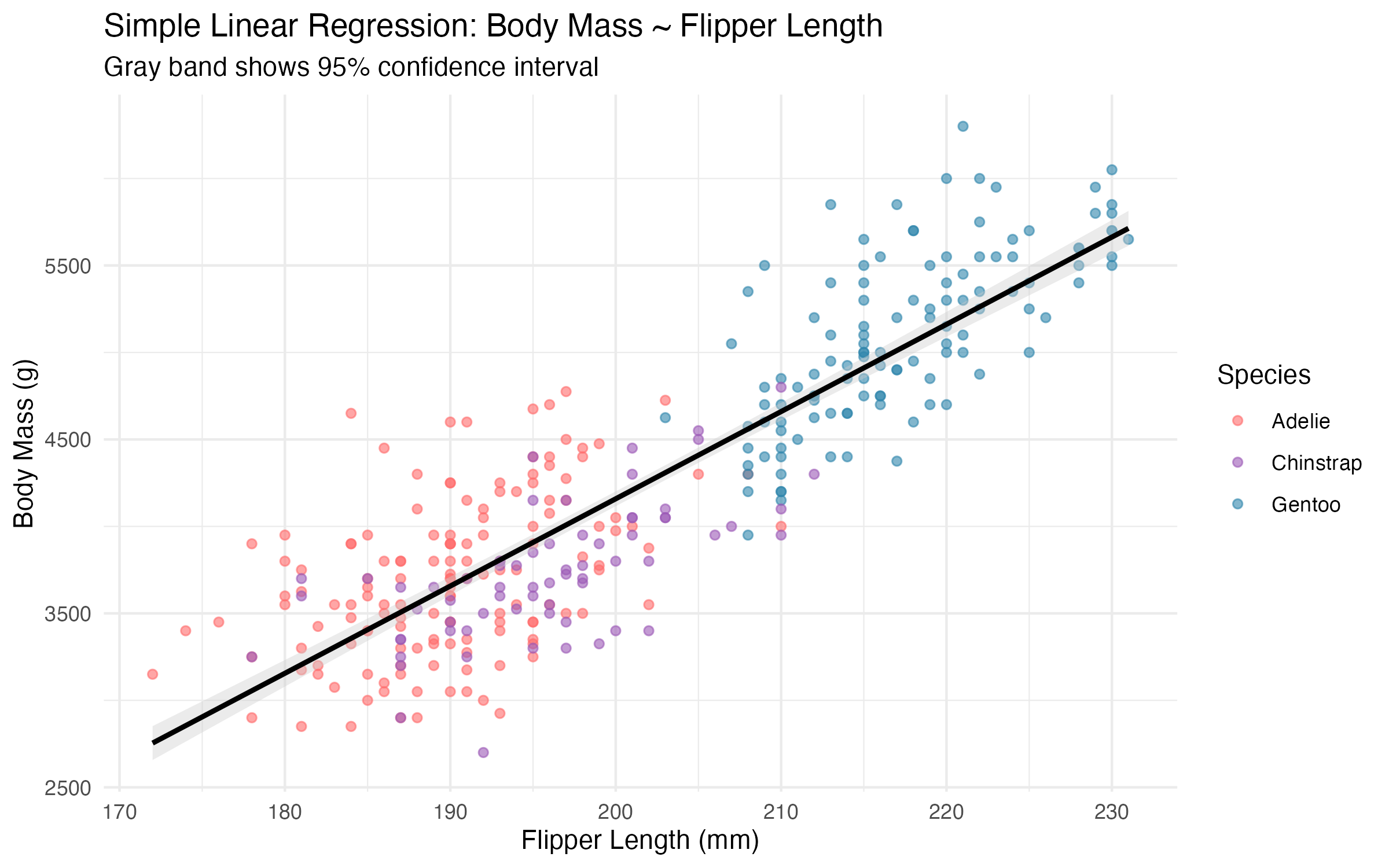
7 Simple Linear Regression

“Time to see if flipper length really predicts our weight!”

7.1 Building and Interpreting the Model

Simple Linear Model Performance

Metric	Value	Interpretation
R²	0.762	76.2% variance explained
RMSE	393.3 g	Mean prediction error
F-statistic	1060.3	p < 0.001 (highly significant)

**Model Equation:**

Body Mass = -5872.1 + 50.2 × Flipper Length

Slope 95% CI: [47.1, 53.2] grams/mm

7.1.0.1 Example Predictions

Predicted Body Mass for Example Flipper Lengths

Flipper Length (mm)	Predicted Body Mass (g)	95% CI Lower	95% CI Upper
180	3637	3589	3685
200	4749	4712	4786
220	5860	5815	5905

Simple linear regression model showing body mass predicted by flipper length with 95% confidence interval

8 Model Limitations and Assumptions

“Wait, we should read the assumptions first!”

Before interpreting our results, we must acknowledge important limitations:

8.1 Statistical Limitations

Model Diagnostic Summary

Assumption	Result	Status
Linearity	Relationship appears approximately linear	✓ Met
Independence	Observations are independent	✓ Met
Normality	Residuals approximately normal	✓ Reasonable
Homoscedasticity	Variance constant across range	⚠ Violated by species
Outliers	5 observations >2.5 SD	⚠ Present
Residual Std. Error	393.3 grams	✓ Acceptable

Model diagnostic plot showing residuals clustered by species, indicating model limitations

8.2 Key Limitations

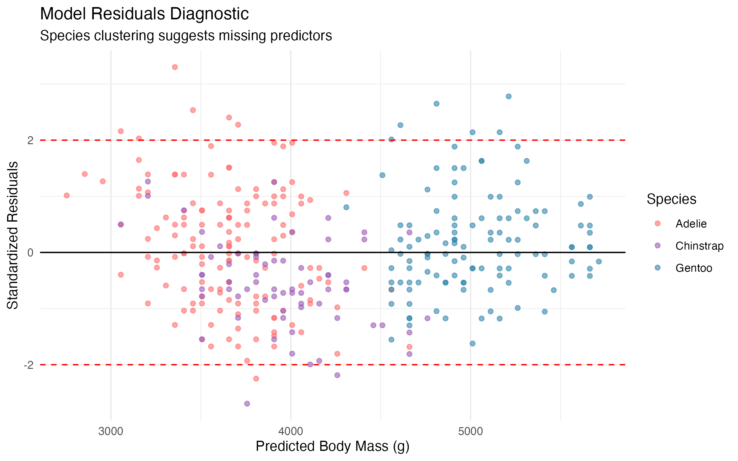
1. Simpson’s Paradox Risk: The model ignores species differences, potentially masking important biological relationships
2. Model Assumptions:
   • Linear relationship assumption appears reasonable
   • Residual clustering by species indicates missing predictors
   • Homoscedasticity assumption may be violated across species
3. Temporal Generalizability: Data spans 2007-2009; climate change may affect current relationships
4. Geographic Scope: Limited to Palmer Station region; may not generalize to other penguin populations
5. Measurement Precision: Morphometric measurements have inherent measurement error not captured in model
6. Biological Constraints: Model predictions outside observed flipper length range (172-231mm) should be interpreted cautiously

9 Practical Applications and Implications

“Now let’s use this model to help our penguin community!”

9.1 Real-World Applications

Our simple regression model has several practical applications in Antarctic research:

Practical Applications of the Model

Application	Description	Relevance
Field Assessment	Flipper measurements estimate body condition (effect size: 0.06)	High
Population Monitoring	Track penguin health trends using morphometric relationships	High
Climate Research	Changes in relationships may indicate environmental stress	Medium
Conservation Planning	Identify underweight individuals for intervention	High

Body Condition Classification Thresholds

Condition Category	Body Mass Range (g)	Percentile
Low Condition	< 3550	Below 25th
Normal Range	3550–4775	25th–75th
High Condition	> 4775	Above 75th

10 Key Findings and Next Steps

10.1 What We’ve Learned in Part 1

1. Strong Predictive Relationship: Flipper length explains 76.2% of body mass variance (R² = 0.762), providing a reliable field assessment tool

2. Species-Specific Patterns: Residual clustering by species suggests important biological differences not captured by flipper length alone

3. Model Performance: RMSE of 393g indicates reasonable prediction accuracy for most applications

4. Research Implications: Simple morphometric relationships can support field research and conservation efforts

10.2 Looking Ahead to Part 2

Our residual analysis reveals clear opportunities for improvement through:

• Species Integration: Accounting for biological differences between penguin species
• Multiple Predictors: Incorporating bill measurements for enhanced accuracy
• Interaction Effects: Exploring how predictors work together
• Model Validation: Comparing simple vs. complex model performance

🎯 Preview: Dramatic Model Improvement

In Part 2, adding species information will improve our model’s R² from 0.762 to over 0.860 - demonstrating why biological context matters in ecological modeling!

11 Reproducibility Information

This blog post is part of a reproducible research compendium using ZZCOLLAB. To reproduce the entire analysis:

11.1 Quick Start

git clone <repository-url>
cd posts/palmerpenguinspart1

# Build Docker environment (one-time setup)
make docker-build

# Run complete analysis pipeline and render blog post
make docker-post-render

# View results
open index.html

11.2 Analysis Pipeline

The complete analysis consists of three reproducible scripts:

1. 01_prepare_data.R - Load Palmer Penguins data, clean, and save derived data
2. 02_fit_models.R - Fit simple linear regression model, extract coefficients and diagnostics
3. 03_generate_figures.R - Generate publication-quality figures from analysis results

All figures shown in this post are generated by the analysis scripts and can be reproduced exactly using the provided code.

11.3 Environment Information

Analysis Environment

R Version	R version 4.5.2 (2025-10-31)
Platform	aarch64-apple-darwin20
Analysis Date	2026-02-10

11.4 Data Source

Palmer Penguins Dataset: - Gorman KB, Williams TD, Fraser WR (2014). Ecological sexual dimorphism and environmental variability within a community of Antarctic penguins (genus Pygoscelis). PLOS ONE 9(3): e90081. - Data accessible via: palmerpenguins R package - Original data repository: https://github.com/allisonhorst/palmerpenguins