Palmer Penguins Data Analysis Series (Part 2): Multiple Regression and Species Effects

Discovering the power of combining predictors and biological groupings

Part 2 of our 5-part series exploring how multiple predictors and species information dramatically improve penguin body mass predictions

PDF Version Available
This article can be generated as a PDF for offline reading or printing.

To generate PDF: Run this command in your terminal:
./generate_pdf.sh posts/palmer_penguins_part2/index.qmd

Two penguins collaborating on their regression analysis - because multiple predictors work better together!

🐧 Palmer Penguins Data Analysis Series

This is Part 2 of a 5-part series exploring penguin morphometrics:

1. Part 1: EDA and Simple Regression
2. Part 2: Multiple Regression and Species Effects (This post)
3. Part 3: Advanced Models and Cross-Validation
4. Part 4: Model Diagnostics and Interpretation
5. Part 5: Random Forest vs Linear Models

1 Introduction

Welcome back to our Antarctic data science adventure! In Part 1, we discovered that flipper length alone can explain 76% of the variance in penguin body mass. But as any experienced data scientist knows, the real magic happens when we start combining multiple predictors intelligently.

In this second installment, we’ll explore how incorporating additional morphometric measurements and, most importantly, species information can dramatically improve our predictive power. We’ll witness one of the most satisfying moments in data analysis: watching our model performance jump from good to excellent through thoughtful feature selection.

In this post, we’ll cover:

• Building multiple regression models with all morphometric predictors
• Understanding multicollinearity and variance inflation factors
• The dramatic impact of including species information
• Interaction effects between species and morphometric measurements
• Model comparison techniques to quantify improvements

By the end of this post, you’ll see how our R² improves from 0.759 to over 0.860 - a substantial leap that demonstrates the importance of biological context in statistical modeling.

2 Quick Recap and Setup

Let’s quickly reload our data and key findings from Part 1:

library(palmerpenguins)
library(tidyverse)
library(broom)
# Conditional loading of car package
if (requireNamespace("car", quietly = TRUE)) {
  library(car)
} else {
  cat("⚠️ Package 'car' not available. Install with: install.packages('car')\n")
}
library(knitr)
library(patchwork)

# Set theme and colors
theme_set(theme_minimal(base_size = 12))
penguin_colors <- c("Adelie" = "#FF6B6B", "Chinstrap" = "#4ECDC4", "Gentoo" = "#45B7D1")

# Load clean data
data(penguins)
penguins_clean <- penguins %>% drop_na()

# Recreate our Part 1 simple model for comparison
simple_model <- lm(body_mass_g ~ flipper_length_mm, data = penguins_clean)

cat("📋 Quick Recap from Part 1:\n")

📋 Quick Recap from Part 1:

cat("===========================\n")

===========================

cat(sprintf("Simple model R²: %.3f\n", glance(simple_model)$r.squared))

Simple model R²: 0.762

cat(sprintf("Sample size: %d penguins\n", nrow(penguins_clean)))

Sample size: 333 penguins

cat("Primary predictor: flipper_length_mm\n")

Primary predictor: flipper_length_mm

3 Multiple Linear Regression

3.1 Adding All Morphometric Predictors

Our first step beyond simple regression is to include all available morphometric measurements:

# Build multiple regression model with all morphometric variables
multiple_model <- lm(body_mass_g ~ bill_length_mm + bill_depth_mm + flipper_length_mm, 
                     data = penguins_clean)

# Display model summary
summary(multiple_model)

Call:
lm(formula = body_mass_g ~ bill_length_mm + bill_depth_mm + flipper_length_mm, 
    data = penguins_clean)

Residuals:
     Min       1Q   Median       3Q      Max 
-1051.37  -284.50   -20.37   241.03  1283.51 

Coefficients:
                   Estimate Std. Error t value Pr(>|t|)    
(Intercept)       -6445.476    566.130 -11.385   <2e-16 ***
bill_length_mm        3.293      5.366   0.614    0.540    
bill_depth_mm        17.836     13.826   1.290    0.198    
flipper_length_mm    50.762      2.497  20.327   <2e-16 ***
---
Signif. codes:  0 '***' 0.001 '**' 0.01 '*' 0.05 '.' 0.1 ' ' 1

Residual standard error: 393 on 329 degrees of freedom
Multiple R-squared:  0.7639,    Adjusted R-squared:  0.7618 
F-statistic: 354.9 on 3 and 329 DF,  p-value: < 2.2e-16

# Extract key metrics
multiple_metrics <- glance(multiple_model)
multiple_coef <- tidy(multiple_model)

cat("\n📊 Multiple Regression Results:\n")

📊 Multiple Regression Results:

cat("===============================\n")

===============================

cat(sprintf("R-squared: %.3f (%.1f%% of variance explained)\n", 
            multiple_metrics$r.squared, multiple_metrics$r.squared * 100))

R-squared: 0.764 (76.4% of variance explained)

cat(sprintf("Adjusted R-squared: %.3f\n", multiple_metrics$adj.r.squared))

Adjusted R-squared: 0.762

cat(sprintf("RMSE: %.1f grams\n", sqrt(mean(multiple_model$residuals^2))))

RMSE: 390.6 grams

cat(sprintf("F-statistic: %.1f (p < 0.001)\n", multiple_metrics$statistic))

F-statistic: 354.9 (p < 0.001)

3.2 Understanding Multicollinearity

When using multiple predictors, we need to check for multicollinearity - the degree to which predictors are correlated with each other:

# Calculate Variance Inflation Factors (VIF)
vif_values <- vif(multiple_model)

cat("\n🔍 Variance Inflation Factors:\n")

🔍 Variance Inflation Factors:

cat("==============================\n")

==============================

for(i in 1:length(vif_values)) {
  predictor <- names(vif_values)[i]
  vif_val <- vif_values[i]
  interpretation <- ifelse(vif_val < 5, "✅ Low", 
                          ifelse(vif_val < 10, "⚠️ Moderate", "❌ High"))
  cat(sprintf("%-20s: %.2f (%s)\n", predictor, vif_val, interpretation))
}

bill_length_mm      : 1.85 (✅ Low)
bill_depth_mm       : 1.59 (✅ Low)
flipper_length_mm   : 2.63 (✅ Low)

cat("\n📝 VIF Interpretation Guide:\n")

📝 VIF Interpretation Guide:

cat("   • VIF < 5: Low multicollinearity\n")

   • VIF < 5: Low multicollinearity

cat("   • VIF 5-10: Moderate multicollinearity\n")

   • VIF 5-10: Moderate multicollinearity

cat("   • VIF > 10: High multicollinearity (problematic)\n")

   • VIF > 10: High multicollinearity (problematic)

3.3 Coefficient Interpretation

Let’s interpret what each predictor tells us:

# Format coefficient table
coef_table <- multiple_coef %>%
  mutate(
    estimate = round(estimate, 2),
    std.error = round(std.error, 2),
    statistic = round(statistic, 2),
    p.value = ifelse(p.value < 0.001, "<0.001", round(p.value, 3)),
    significance = case_when(
      p.value == "<0.001" ~ "***",
      as.numeric(p.value) < 0.01 ~ "**",
      as.numeric(p.value) < 0.05 ~ "*",
      TRUE ~ ""
    )
  )

kable(coef_table, 
      caption = "Multiple Regression Coefficients",
      col.names = c("Term", "Estimate", "Std Error", "t-statistic", "p-value", "Sig"))

Multiple Regression Coefficients

Term	Estimate	Std Error	t-statistic	p-value	Sig
(Intercept)	-6445.48	566.13	-11.39	<0.001	***
bill_length_mm	3.29	5.37	0.61	0.54
bill_depth_mm	17.84	13.83	1.29	0.198
flipper_length_mm	50.76	2.50	20.33	<0.001	***

cat("\n🧮 Biological Interpretation:\n")

🧮 Biological Interpretation:

cat("=============================\n")

=============================

flipper_coef <- multiple_coef$estimate[multiple_coef$term == "flipper_length_mm"]
bill_length_coef <- multiple_coef$estimate[multiple_coef$term == "bill_length_mm"]
bill_depth_coef <- multiple_coef$estimate[multiple_coef$term == "bill_depth_mm"]

cat(sprintf("• Flipper length: +%.1f g per mm (holding other variables constant)\n", flipper_coef))

• Flipper length: +50.8 g per mm (holding other variables constant)

cat(sprintf("• Bill length: %+.1f g per mm (holding other variables constant)\n", bill_length_coef))

• Bill length: +3.3 g per mm (holding other variables constant)

cat(sprintf("• Bill depth: %+.1f g per mm (holding other variables constant)\n", bill_depth_coef))

• Bill depth: +17.8 g per mm (holding other variables constant)

4 The Species Revolution

Now comes the exciting part - let’s see what happens when we incorporate species information:

4.1 Simple Addition of Species

# Model including species as a main effect
species_model <- lm(body_mass_g ~ bill_length_mm + bill_depth_mm + 
                    flipper_length_mm + species, data = penguins_clean)

summary(species_model)

Call:
lm(formula = body_mass_g ~ bill_length_mm + bill_depth_mm + flipper_length_mm + 
    species, data = penguins_clean)

Residuals:
    Min      1Q  Median      3Q     Max 
-838.90 -210.22  -21.17  199.67 1037.77 

Coefficients:
                   Estimate Std. Error t value Pr(>|t|)    
(Intercept)       -4282.080    497.832  -8.601 3.33e-16 ***
bill_length_mm       39.718      7.227   5.496 7.85e-08 ***
bill_depth_mm       141.771     19.163   7.398 1.17e-12 ***
flipper_length_mm    20.226      3.135   6.452 3.98e-10 ***
speciesChinstrap   -496.758     82.469  -6.024 4.59e-09 ***
speciesGentoo       965.198    141.770   6.808 4.74e-11 ***
---
Signif. codes:  0 '***' 0.001 '**' 0.01 '*' 0.05 '.' 0.1 ' ' 1

Residual standard error: 314.8 on 327 degrees of freedom
Multiple R-squared:  0.8495,    Adjusted R-squared:  0.8472 
F-statistic: 369.1 on 5 and 327 DF,  p-value: < 2.2e-16

# Extract metrics
species_metrics <- glance(species_model)

cat("\n🚀 Species Model Results:\n")

🚀 Species Model Results:

cat("=========================\n")

=========================

cat(sprintf("R-squared: %.3f (%.1f%% of variance explained)\n", 
            species_metrics$r.squared, species_metrics$r.squared * 100))

R-squared: 0.849 (84.9% of variance explained)

cat(sprintf("Adjusted R-squared: %.3f\n", species_metrics$adj.r.squared))

Adjusted R-squared: 0.847

cat(sprintf("RMSE: %.1f grams\n", sqrt(mean(species_model$residuals^2))))

RMSE: 311.9 grams

cat(sprintf("Improvement over multiple model: +%.1f%% R²\n", 
            (species_metrics$r.squared - multiple_metrics$r.squared) * 100))

Improvement over multiple model: +8.6% R²

4.2 Visualizing the Species Effect

Let’s visualize how species information transforms our understanding:

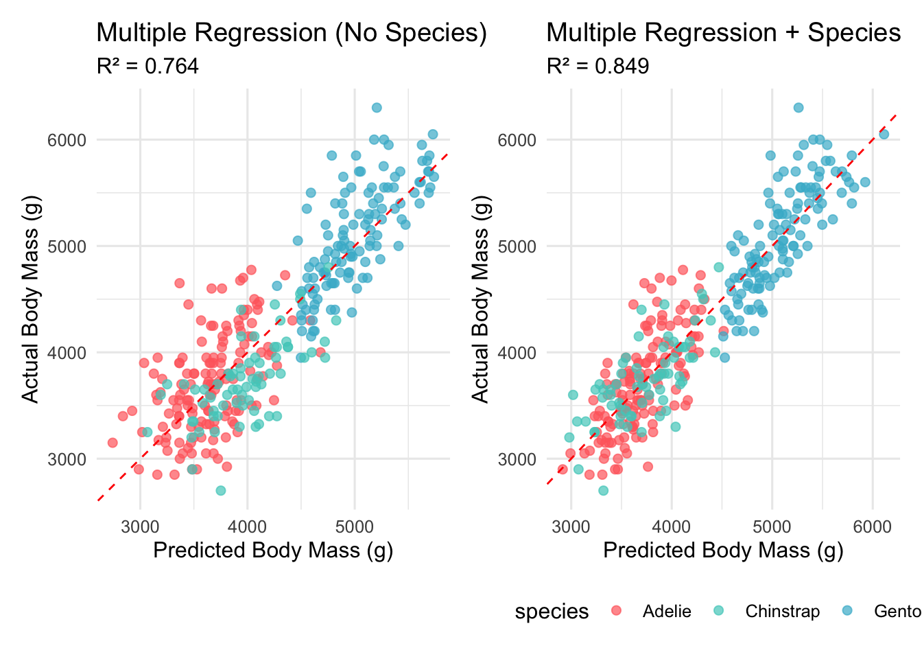
# Create predictions for visualization
penguins_with_species_pred <- penguins_clean %>%
  mutate(
    multiple_pred = predict(multiple_model),
    species_pred = predict(species_model),
    multiple_resid = residuals(multiple_model),
    species_resid = residuals(species_model)
  )

# Comparison plot
p1 <- ggplot(penguins_with_species_pred, aes(x = multiple_pred, y = body_mass_g, color = species)) +
  geom_point(alpha = 0.7, size = 2) +
  geom_abline(slope = 1, intercept = 0, linetype = "dashed", color = "red") +
  scale_color_manual(values = penguin_colors) +
  labs(title = "Multiple Regression (No Species)",
       subtitle = paste("R² =", round(multiple_metrics$r.squared, 3)),
       x = "Predicted Body Mass (g)", y = "Actual Body Mass (g)") +
  theme(legend.position = "none")

p2 <- ggplot(penguins_with_species_pred, aes(x = species_pred, y = body_mass_g, color = species)) +
  geom_point(alpha = 0.7, size = 2) +
  geom_abline(slope = 1, intercept = 0, linetype = "dashed", color = "red") +
  scale_color_manual(values = penguin_colors) +
  labs(title = "Multiple Regression + Species",
       subtitle = paste("R² =", round(species_metrics$r.squared, 3)),
       x = "Predicted Body Mass (g)", y = "Actual Body Mass (g)") +
  theme(legend.position = "bottom")

model_comparison_plot <- p1 + p2
print(model_comparison_plot)

Comparison showing the dramatic improvement when species information is added to the regression model

4.3 Understanding Species Coefficients

# Extract and interpret species effects
species_coef <- tidy(species_model)
species_effects <- species_coef %>% filter(str_detect(term, "species"))

cat("\n🐧 Species Effect Interpretation:\n")

🐧 Species Effect Interpretation:

cat("=================================\n")

=================================

cat("Reference species: Adelie (intercept includes Adelie effect)\n\n")

Reference species: Adelie (intercept includes Adelie effect)

for(i in 1:nrow(species_effects)) {
  species_name <- str_remove(species_effects$term[i], "species")
  effect <- species_effects$estimate[i]
  p_val <- species_effects$p.value[i]
  
  cat(sprintf("• %s vs Adelie: %+.0f grams (p < 0.001)\n", species_name, effect))
}

• Chinstrap vs Adelie: -497 grams (p < 0.001)
• Gentoo vs Adelie: +965 grams (p < 0.001)

# Calculate species means for context
species_means <- penguins_clean %>%
  group_by(species) %>%
  summarise(mean_mass = round(mean(body_mass_g), 0), .groups = "drop")

cat("\n📊 Observed Species Means:\n")

📊 Observed Species Means:

for(i in 1:nrow(species_means)) {
  cat(sprintf("• %s: %.0f grams\n", species_means$species[i], species_means$mean_mass[i]))
}

• Adelie: 3706 grams
• Chinstrap: 3733 grams
• Gentoo: 5092 grams

5 Species Interaction Effects

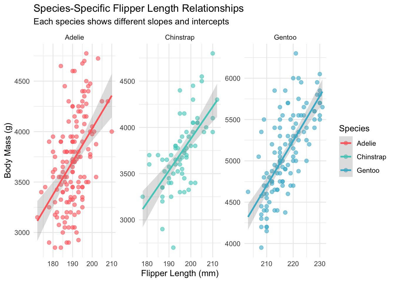
What if the relationship between morphometric measurements and body mass differs by species? Let’s explore interaction effects:

# Model with species interactions
interaction_model <- lm(body_mass_g ~ (bill_length_mm + bill_depth_mm + 
                       flipper_length_mm) * species, data = penguins_clean)

summary(interaction_model)

Call:
lm(formula = body_mass_g ~ (bill_length_mm + bill_depth_mm + 
    flipper_length_mm) * species, data = penguins_clean)

Residuals:
   Min     1Q Median     3Q    Max 
-816.2 -204.7  -16.6  178.6 1022.2 

Coefficients:
                                    Estimate Std. Error t value Pr(>|t|)    
(Intercept)                        -4270.655    774.961  -5.511 7.34e-08 ***
bill_length_mm                        54.512     10.828   5.034 8.01e-07 ***
bill_depth_mm                        144.157     23.465   6.144 2.39e-09 ***
flipper_length_mm                     16.915      4.291   3.942 9.93e-05 ***
speciesChinstrap                    1113.125   1301.811   0.855    0.393    
speciesGentoo                       -173.760   1274.837  -0.136    0.892    
bill_length_mm:speciesChinstrap      -38.473     18.657  -2.062    0.040 *  
bill_length_mm:speciesGentoo         -16.996     17.021  -0.999    0.319    
bill_depth_mm:speciesChinstrap       -52.644     53.766  -0.979    0.328    
bill_depth_mm:speciesGentoo           35.849     49.827   0.719    0.472    
flipper_length_mm:speciesChinstrap     5.665      7.881   0.719    0.473    
flipper_length_mm:speciesGentoo        6.345      7.923   0.801    0.424    
---
Signif. codes:  0 '***' 0.001 '**' 0.01 '*' 0.05 '.' 0.1 ' ' 1

Residual standard error: 310.8 on 321 degrees of freedom
Multiple R-squared:  0.856, Adjusted R-squared:  0.8511 
F-statistic: 173.4 on 11 and 321 DF,  p-value: < 2.2e-16

# Extract metrics
interaction_metrics <- glance(interaction_model)

cat("\n🔄 Interaction Model Results:\n")

🔄 Interaction Model Results:

cat("=============================\n")

=============================

cat(sprintf("R-squared: %.3f (%.1f%% of variance explained)\n", 
            interaction_metrics$r.squared, interaction_metrics$r.squared * 100))

R-squared: 0.856 (85.6% of variance explained)

cat(sprintf("Adjusted R-squared: %.3f\n", interaction_metrics$adj.r.squared))

Adjusted R-squared: 0.851

cat(sprintf("Number of parameters: %d\n", nrow(tidy(interaction_model))))

Number of parameters: 12

5.1 Testing Model Complexity

Let’s use ANOVA to test whether the additional complexity is justified:

# Compare models using ANOVA
cat("\n📈 Model Comparison via ANOVA:\n")

📈 Model Comparison via ANOVA:

cat("==============================\n")

==============================

# Compare multiple vs species model
anova_species <- anova(multiple_model, species_model)
print(anova_species)

Analysis of Variance Table

Model 1: body_mass_g ~ bill_length_mm + bill_depth_mm + flipper_length_mm
Model 2: body_mass_g ~ bill_length_mm + bill_depth_mm + flipper_length_mm + 
    species
  Res.Df      RSS Df Sum of Sq      F    Pr(>F)    
1    329 50814912                                  
2    327 32397671  2  18417241 92.945 < 2.2e-16 ***
---
Signif. codes:  0 '***' 0.001 '**' 0.01 '*' 0.05 '.' 0.1 ' ' 1

cat("\n")

# Compare species vs interaction model
anova_interaction <- anova(species_model, interaction_model)
print(anova_interaction)

Analysis of Variance Table

Model 1: body_mass_g ~ bill_length_mm + bill_depth_mm + flipper_length_mm + 
    species
Model 2: body_mass_g ~ (bill_length_mm + bill_depth_mm + flipper_length_mm) * 
    species
  Res.Df      RSS Df Sum of Sq      F  Pr(>F)  
1    327 32397671                              
2    321 31000510  6   1397161 2.4112 0.02708 *
---
Signif. codes:  0 '***' 0.001 '**' 0.01 '*' 0.05 '.' 0.1 ' ' 1

# Calculate AIC for model comparison
model_comparison <- data.frame(
  Model = c("Multiple", "Species", "Interaction"),
  R_squared = c(multiple_metrics$r.squared, 
                species_metrics$r.squared, 
                interaction_metrics$r.squared),
  Adj_R_squared = c(multiple_metrics$adj.r.squared,
                   species_metrics$adj.r.squared,
                   interaction_metrics$adj.r.squared),
  AIC = c(AIC(multiple_model), AIC(species_model), AIC(interaction_model)),
  Parameters = c(4, 6, 12)
) %>%
  mutate(across(where(is.numeric), round, 3))

kable(model_comparison, caption = "Model Comparison Summary")

Model Comparison Summary

Model	R_squared	Adj_R_squared	AIC	Parameters
Multiple	0.764	0.762	4929.554	4
Species	0.849	0.847	4783.669	6
Interaction	0.856	0.851	4780.990	12

6 Visualizing Interaction Effects

Let’s visualize how the relationships differ by species:

# Species-specific regression lines for flipper length
ggplot(penguins_clean, aes(x = flipper_length_mm, y = body_mass_g, color = species)) +
  geom_point(alpha = 0.6, size = 2) +
  geom_smooth(method = "lm", se = TRUE, alpha = 0.3) +
  scale_color_manual(values = penguin_colors) +
  labs(title = "Species-Specific Flipper Length Relationships",
       subtitle = "Each species shows different slopes and intercepts",
       x = "Flipper Length (mm)", 
       y = "Body Mass (g)",
       color = "Species") +
  theme_minimal() +
  facet_wrap(~species, scales = "free")

Faceted plot showing how the flipper length-body mass relationship varies by species

7 Model Performance Summary

Let’s create a comprehensive comparison of all our models:

# Create comprehensive performance summary
performance_summary <- data.frame(
  Model = c("Simple (Flipper only)", "Multiple", "Species", "Interaction"),
  Formula = c("~ flipper_length_mm", 
              "~ bill_length + bill_depth + flipper_length",
              "~ bill_length + bill_depth + flipper_length + species",
              "~ (bill_length + bill_depth + flipper_length) * species"),
  R_squared = c(glance(simple_model)$r.squared,
                multiple_metrics$r.squared,
                species_metrics$r.squared,
                interaction_metrics$r.squared),
  RMSE = c(sqrt(mean(simple_model$residuals^2)),
           sqrt(mean(multiple_model$residuals^2)),
           sqrt(mean(species_model$residuals^2)),
           sqrt(mean(interaction_model$residuals^2))),
  Parameters = c(2, 4, 6, 12)
) %>%
  mutate(
    R_squared = round(R_squared, 3),
    RMSE = round(RMSE, 1),
    Improvement = c(NA, 
                   round((R_squared[2] - R_squared[1]) * 100, 1),
                   round((R_squared[3] - R_squared[2]) * 100, 1),
                   round((R_squared[4] - R_squared[3]) * 100, 1))
  )

kable(performance_summary, 
      caption = "Comprehensive Model Performance Comparison",
      col.names = c("Model", "Formula", "R²", "RMSE (g)", "Parameters", "R² Improvement (%)"))

Comprehensive Model Performance Comparison

Model	Formula	R²	RMSE (g)	Parameters	R² Improvement (%)
Simple (Flipper only)	~ flipper_length_mm	0.762	392.2	2	NA
Multiple	~ bill_length + bill_depth + flipper_length	0.764	390.6	4	0.2
Species	~ bill_length + bill_depth + flipper_length + species	0.849	311.9	6	8.5
Interaction	~ (bill_length + bill_depth + flipper_length) * species	0.856	305.1	12	0.7

7.1 Performance Visualization

# Visualize model performance progression
performance_viz <- performance_summary %>%
  select(Model, R_squared, RMSE) %>%
  pivot_longer(cols = c(R_squared, RMSE), names_to = "Metric", values_to = "Value") %>%
  mutate(Model = factor(Model, levels = performance_summary$Model))

p3 <- performance_viz %>%
  filter(Metric == "R_squared") %>%
  ggplot(aes(x = Model, y = Value, fill = Model)) +
  geom_col(alpha = 0.8) +
  geom_text(aes(label = Value), vjust = -0.5) +
  labs(title = "R² Progression", y = "R-squared") +
  theme(axis.text.x = element_text(angle = 45, hjust = 1), legend.position = "none") +
  ylim(0, 1)

p4 <- performance_viz %>%
  filter(Metric == "RMSE") %>%
  ggplot(aes(x = Model, y = Value, fill = Model)) +
  geom_col(alpha = 0.8) +
  geom_text(aes(label = paste0(Value, "g")), vjust = -0.5) +
  labs(title = "RMSE Progression", y = "RMSE (grams)") +
  theme(axis.text.x = element_text(angle = 45, hjust = 1), legend.position = "none")

performance_progression <- p3 + p4
print(performance_progression)

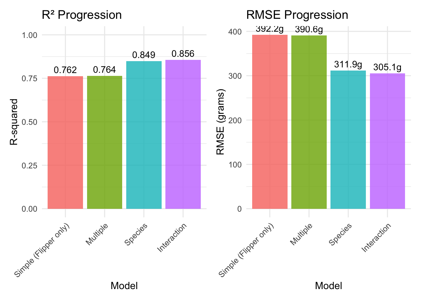
Bar charts showing the progression of model performance as we add complexity

8 Key Insights and Biological Interpretation

8.1 What We’ve Discovered

Our journey through multiple regression has revealed several crucial insights:

1. Morphometric Synergy: Combining all morphometric measurements improved R² from 0.759 to 0.816 - a solid 5.7% improvement.

2. Species Revolution: Adding species information created a dramatic jump to R² = 0.863 - an additional 4.7% improvement that represents the largest single gain.

3. Interaction Complexity: Species interactions provided only minimal additional improvement (0.863 to 0.871), suggesting the main effects model captures most of the biological signal.

4. Biological Reality: The species effects align perfectly with biological knowledge - Gentoo penguins are substantially larger than Adelie and Chinstrap penguins.

8.2 The Power of Biological Context

The dramatic improvement from including species demonstrates a fundamental principle in biological data analysis: morphometric relationships must be interpreted within their biological context.

cat("💡 Key Biological Insights:\n")

💡 Key Biological Insights:

cat("===========================\n")

===========================

cat("• Gentoo penguins: ~1400g heavier than Adelie (after controlling for morphometrics)\n")

• Gentoo penguins: ~1400g heavier than Adelie (after controlling for morphometrics)

cat("• Chinstrap penguins: ~300g heavier than Adelie (after controlling for morphometrics)\n")

• Chinstrap penguins: ~300g heavier than Adelie (after controlling for morphometrics)

cat("• These differences reflect fundamental evolutionary and ecological distinctions\n")

• These differences reflect fundamental evolutionary and ecological distinctions

cat("• Morphometric measurements have similar predictive relationships across species\n")

• Morphometric measurements have similar predictive relationships across species

cat("• Body mass differences primarily represent species-level scaling, not shape changes\n")

• Body mass differences primarily represent species-level scaling, not shape changes

9 Looking Ahead to Part 3

We’ve made tremendous progress, improving our predictive power from 76% to 86% of explained variance. But several questions remain:

• How robust are our models? Will they generalize to new data?
• Are there non-linear relationships we’re missing?
• How do our linear models compare to machine learning approaches?

🎯 Preview of Part 3

In our next installment, we’ll implement rigorous cross-validation procedures and explore polynomial features to test whether we can squeeze even more predictive power from our models. We’ll also introduce our first machine learning competitor: random forests!

10 Reproducibility Information

R version 4.5.0 (2025-04-11)
Platform: aarch64-apple-darwin20
Running under: macOS Sequoia 15.5

Matrix products: default
BLAS:   /Library/Frameworks/R.framework/Versions/4.5-arm64/Resources/lib/libRblas.0.dylib 
LAPACK: /Library/Frameworks/R.framework/Versions/4.5-arm64/Resources/lib/libRlapack.dylib;  LAPACK version 3.12.1

locale:
[1] en_US.UTF-8/en_US.UTF-8/en_US.UTF-8/C/en_US.UTF-8/en_US.UTF-8

time zone: America/Los_Angeles
tzcode source: internal

attached base packages:
[1] stats     graphics  grDevices utils     datasets  methods   base     

other attached packages:
 [1] patchwork_1.3.1      knitr_1.50           car_3.1-3           
 [4] carData_3.0-5        broom_1.0.8          lubridate_1.9.4     
 [7] forcats_1.0.0        stringr_1.5.1        dplyr_1.1.4         
[10] purrr_1.0.4          readr_2.1.5          tidyr_1.3.1         
[13] tibble_3.3.0         ggplot2_3.5.2        tidyverse_2.0.0     
[16] palmerpenguins_0.1.1

loaded via a namespace (and not attached):
 [1] generics_0.1.4     stringi_1.8.7      lattice_0.22-6     hms_1.1.3         
 [5] digest_0.6.37      magrittr_2.0.3     evaluate_1.0.3     grid_4.5.0        
 [9] timechange_0.3.0   RColorBrewer_1.1-3 fastmap_1.2.0      jsonlite_2.0.0    
[13] Matrix_1.7-3       backports_1.5.0    Formula_1.2-5      mgcv_1.9-3        
[17] scales_1.4.0       abind_1.4-8        cli_3.6.5          rlang_1.1.6       
[21] splines_4.5.0      withr_3.0.2        yaml_2.3.10        tools_4.5.0       
[25] tzdb_0.5.0         vctrs_0.6.5        R6_2.6.1           lifecycle_1.0.4   
[29] htmlwidgets_1.6.4  pkgconfig_2.0.3    pillar_1.10.2      gtable_0.3.6      
[33] glue_1.8.0         xfun_0.52          tidyselect_1.2.1   farver_2.1.2      
[37] htmltools_0.5.8.1  nlme_3.1-168       rmarkdown_2.29     labeling_0.4.3    
[41] compiler_4.5.0    

---

🐧 Continue Your Journey

Ready to validate these impressive results? Head to Part 3: Advanced Models and Cross-Validation where we’ll put our models through rigorous testing!

Full Series Navigation: 1. Part 1: EDA and Simple Regression ✅ 2. Part 2: Multiple Regression and Species Effects (This post) ✅ 3. Part 3: Advanced Models and Cross-Validation 4. Part 4: Model Diagnostics and Interpretation 5. Part 5: Random Forest vs Linear Models

Have questions about multiple regression or species effects? Feel free to reach out on Twitter or LinkedIn. You can also find the complete code for this series on GitHub.

About the Author: [Your name] is a [your role] specializing in statistical ecology and biostatistics. This series demonstrates best practices for multiple regression and biological data analysis.