Palmer Penguins Data Analysis Series (Part 4): Model Diagnostics and Interpretation

Ensuring our models meet assumptions and understanding what they really tell us

Part 4 of our 5-part series focusing on rigorous diagnostic procedures, assumption checking, and biological interpretation of our penguin models

PDF Version Available
This article can be generated as a PDF for offline reading or printing.

To generate PDF: Run this command in your terminal:
./generate_pdf.sh posts/palmer_penguins_part4/index.qmd

A penguin scientist with a magnifying glass, carefully examining model diagnostics and residual plots!

🐧 Palmer Penguins Data Analysis Series

This is Part 4 of a 5-part series exploring penguin morphometrics:

1. Part 1: EDA and Simple Regression
2. Part 2: Multiple Regression and Species Effects
3. Part 3: Advanced Models and Cross-Validation
4. Part 4: Model Diagnostics and Interpretation (This post)
5. Part 5: Random Forest vs Linear Models

1 Introduction

Welcome to the fourth chapter of our Palmer penguins journey! In Part 3, we validated our models through rigorous cross-validation and confirmed that our species-aware linear model offers excellent predictive performance. But excellent performance doesn’t automatically mean our model is appropriate or that our assumptions are satisfied.

Today, we dive into the critical but often overlooked world of model diagnostics. Think of this as taking your high-performing car to a mechanic - it might run well, but are there underlying issues that could cause problems? In statistical modeling, diagnostic procedures help us understand whether our model is not just performing well, but performing well for the right reasons.

In this post, we’ll explore:

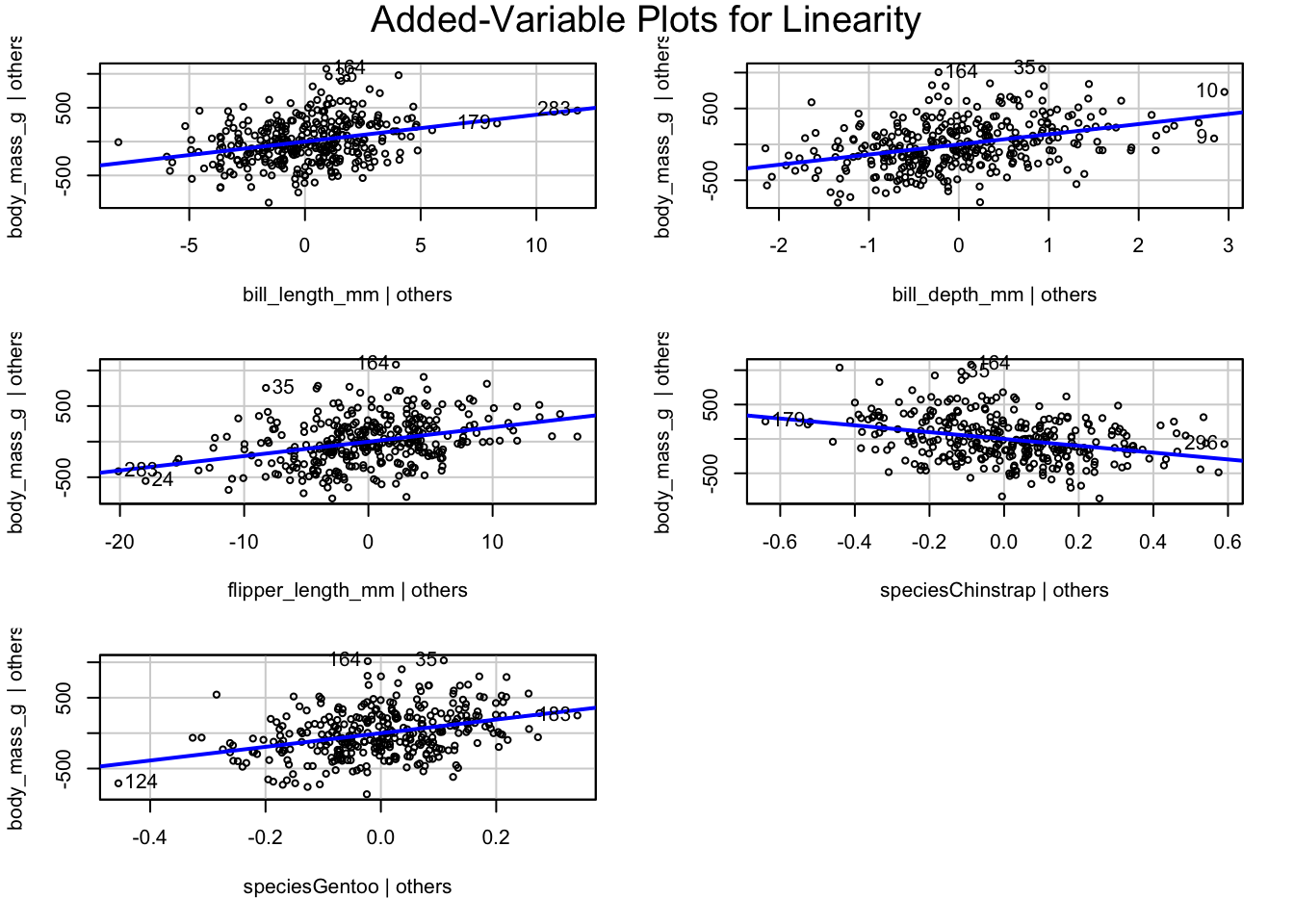
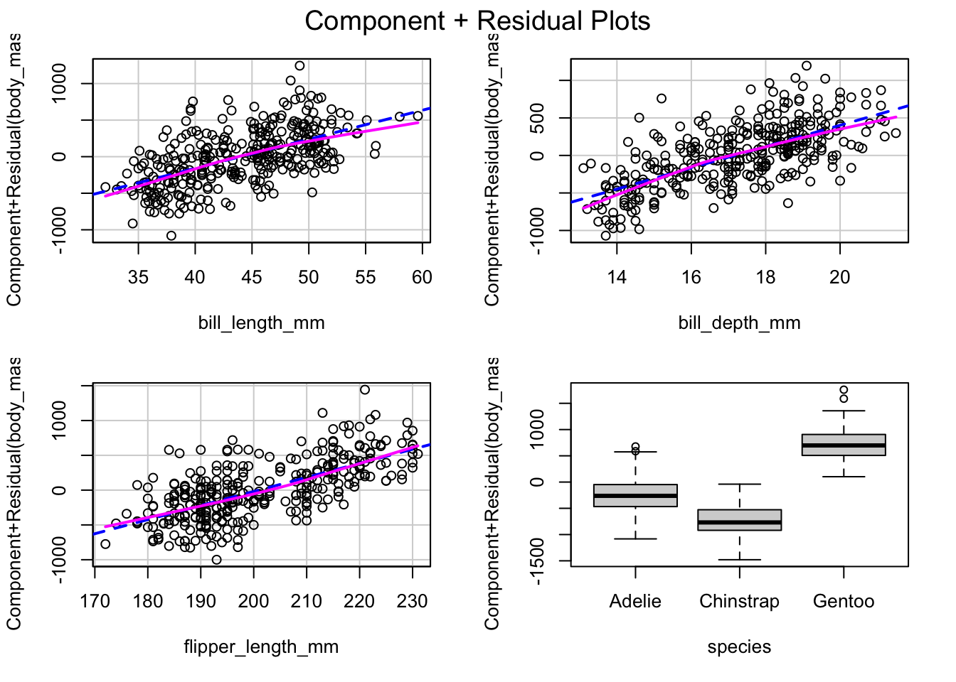
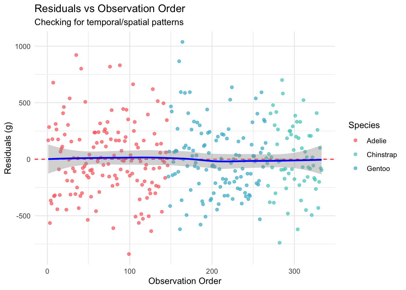
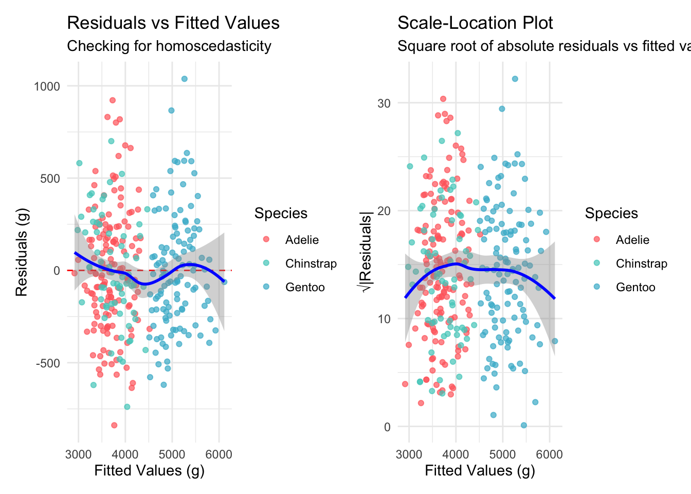
• Comprehensive residual analysis and assumption checking
• Influence diagnostics to identify problematic observations
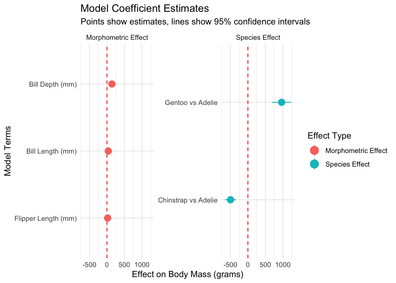
• Biological interpretation of model coefficients
• Prediction intervals and uncertainty quantification
• Best practices for model reporting in ecological research

By the end of this post, you’ll have confidence that your model is not just accurate, but statistically sound and biologically meaningful.

2 Setup and Model Preparation

Let’s reconstruct our best-performing model and prepare for diagnostic analysis:

library(palmerpenguins)
library(tidyverse)
library(broom)
# Conditional loading of optional packages
optional_diagnostic_packages <- c("car", "performance", "see", "lmtest")
for (pkg in optional_diagnostic_packages) {
  if (requireNamespace(pkg, quietly = TRUE)) {
    library(pkg, character.only = TRUE)
  } else {
    cat("⚠️ Package '", pkg, "' not available. Install with: install.packages('", pkg, "')\n")
  }
}
library(knitr)
library(patchwork)

# Set theme and colors
theme_set(theme_minimal(base_size = 12))
penguin_colors <- c("Adelie" = "#FF6B6B", "Chinstrap" = "#4ECDC4", "Gentoo" = "#45B7D1")

# Load and prepare data
data(penguins)
penguins_clean <- penguins %>% drop_na()

# Recreate our best model from previous parts
best_model <- lm(body_mass_g ~ bill_length_mm + bill_depth_mm + 
                 flipper_length_mm + species, data = penguins_clean)

# Add fitted values and residuals to our dataset
penguins_diagnostics <- penguins_clean %>%
  mutate(
    fitted_values = fitted(best_model),
    residuals = residuals(best_model),
    standardized_residuals = rstandard(best_model),
    studentized_residuals = rstudent(best_model),
    leverage = hatvalues(best_model),
    cooks_distance = cooks.distance(best_model)
  )

cat("🔧 Model Diagnostic Setup:\n")

🔧 Model Diagnostic Setup:

cat("==========================\n")

==========================

cat(sprintf("Model: body_mass_g ~ bill_length_mm + bill_depth_mm + flipper_length_mm + species\n"))

Model: body_mass_g ~ bill_length_mm + bill_depth_mm + flipper_length_mm + species

cat(sprintf("Observations: %d\n", nrow(penguins_clean)))

Observations: 333

cat(sprintf("Parameters: %d\n", length(coef(best_model))))

Parameters: 6

cat(sprintf("R-squared: %.3f\n", summary(best_model)$r.squared))

R-squared: 0.849

3 Classical Regression Assumptions

Linear regression relies on several key assumptions. Let’s check each systematically:

3.1 1. Linearity

The relationship between predictors and response should be linear:

# Check linearity using partial residual plots
par(mfrow = c(2, 2))
avPlots(best_model, main = "Added-Variable Plots for Linearity")

par(mfrow = c(1, 1))

# Alternative: Component + residual plots
crPlots(best_model, main = "Component + Residual Plots")

Added-variable plots showing the linear relationships between predictors and response after accounting for other variables

3.2 2. Independence of Residuals

We’ll check for patterns that might indicate dependence:

# Plot residuals vs order (temporal/spatial independence)
penguins_diagnostics <- penguins_diagnostics %>%
  mutate(observation_order = row_number())

p1 <- ggplot(penguins_diagnostics, aes(x = observation_order, y = residuals)) +
  geom_point(aes(color = species), alpha = 0.7) +
  geom_hline(yintercept = 0, linetype = "dashed", color = "red") +
  geom_smooth(method = "loess", se = TRUE, color = "blue") +
  scale_color_manual(values = penguin_colors) +
  labs(title = "Residuals vs Observation Order",
       subtitle = "Checking for temporal/spatial patterns",
       x = "Observation Order", y = "Residuals (g)",
       color = "Species") +
  theme_minimal()

print(p1)

# Durbin-Watson test for autocorrelation
dw_test <- durbinWatsonTest(best_model)
cat("\n📊 Durbin-Watson Test for Autocorrelation:\n")

📊 Durbin-Watson Test for Autocorrelation:

cat("==========================================\n")

==========================================

cat(sprintf("DW Statistic: %.3f\n", dw_test$dw))

DW Statistic: 2.248

cat(sprintf("p-value: %.3f\n", dw_test$p))

p-value: 0.038

cat("Interpretation: Values near 2 indicate no autocorrelation\n")

Interpretation: Values near 2 indicate no autocorrelation

Plot showing residuals versus observation order to check for temporal or spatial dependencies

3.3 3. Homoscedasticity (Constant Variance)

Residual variance should be constant across fitted values:

# Residuals vs fitted values plot
p2 <- ggplot(penguins_diagnostics, aes(x = fitted_values, y = residuals)) +
  geom_point(aes(color = species), alpha = 0.7) +
  geom_hline(yintercept = 0, linetype = "dashed", color = "red") +
  geom_smooth(method = "loess", se = TRUE, color = "blue") +
  scale_color_manual(values = penguin_colors) +
  labs(title = "Residuals vs Fitted Values",
       subtitle = "Checking for homoscedasticity",
       x = "Fitted Values (g)", y = "Residuals (g)",
       color = "Species") +
  theme_minimal()

# Scale-Location plot (sqrt of absolute residuals)
p3 <- ggplot(penguins_diagnostics, aes(x = fitted_values, y = sqrt(abs(residuals)))) +
  geom_point(aes(color = species), alpha = 0.7) +
  geom_smooth(method = "loess", se = TRUE, color = "blue") +
  scale_color_manual(values = penguin_colors) +
  labs(title = "Scale-Location Plot",
       subtitle = "Square root of absolute residuals vs fitted values",
       x = "Fitted Values (g)", y = "√|Residuals|",
       color = "Species") +
  theme_minimal()

homoscedasticity_plots <- p2 + p3
print(homoscedasticity_plots)

# Breusch-Pagan test for heteroscedasticity
bp_test <- bptest(best_model)
cat("\n📊 Breusch-Pagan Test for Heteroscedasticity:\n")

📊 Breusch-Pagan Test for Heteroscedasticity:

cat("==============================================\n")

==============================================

cat(sprintf("BP Statistic: %.3f\n", bp_test$statistic))

BP Statistic: 2.583

cat(sprintf("p-value: %.3f\n", bp_test$p.value))

p-value: 0.764

cat("Interpretation: p > 0.05 suggests constant variance (homoscedasticity)\n")

Interpretation: p > 0.05 suggests constant variance (homoscedasticity)

Diagnostic plots for checking homoscedasticity assumption through residuals vs fitted values

3.4 4. Normality of Residuals

Residuals should follow a normal distribution:

# Q-Q plot for normality
p4 <- ggplot(penguins_diagnostics, aes(sample = standardized_residuals)) +
  stat_qq(aes(color = species), alpha = 0.7) +
  stat_qq_line(color = "red", linetype = "dashed") +
  scale_color_manual(values = penguin_colors) +
  labs(title = "Q-Q Plot of Standardized Residuals",
       subtitle = "Checking normality assumption",
       x = "Theoretical Quantiles", y = "Sample Quantiles",
       color = "Species") +
  theme_minimal()

# Histogram of residuals
p5 <- ggplot(penguins_diagnostics, aes(x = residuals)) +
  geom_histogram(aes(y = after_stat(density)), bins = 30, 
                 fill = "lightblue", alpha = 0.7, color = "white") +
  geom_density(color = "blue", size = 1) +
  stat_function(fun = dnorm, 
                args = list(mean = mean(penguins_diagnostics$residuals), 
                           sd = sd(penguins_diagnostics$residuals)),
                color = "red", linetype = "dashed", size = 1) +
  labs(title = "Distribution of Residuals",
       subtitle = "Blue = actual density, Red = normal distribution",
       x = "Residuals (g)", y = "Density") +
  theme_minimal()

normality_plots <- p4 + p5
print(normality_plots)

# Shapiro-Wilk test for normality
shapiro_test <- shapiro.test(residuals(best_model))
cat("\n📊 Shapiro-Wilk Test for Normality:\n")

📊 Shapiro-Wilk Test for Normality:

cat("====================================\n")

====================================

cat(sprintf("W Statistic: %.4f\n", shapiro_test$statistic))

W Statistic: 0.9921

cat(sprintf("p-value: %.4f\n", shapiro_test$p.value))

p-value: 0.0746

cat("Interpretation: p > 0.05 suggests residuals are normally distributed\n")

Interpretation: p > 0.05 suggests residuals are normally distributed

# Alternative: Anderson-Darling test (more powerful for large samples)
# Install nortest if needed: install.packages("nortest")
if (requireNamespace("nortest", quietly = TRUE)) {
  library(nortest)
  ad_test <- ad.test(residuals(best_model))
  cat(sprintf("\nAnderson-Darling Test p-value: %.4f\n", ad_test$p.value))
} else {
  cat("\n⚠️ nortest package not available. Install with: install.packages('nortest')\n")
  cat("Using Shapiro-Wilk test results instead.\n")
}

⚠️ nortest package not available. Install with: install.packages('nortest')
Using Shapiro-Wilk test results instead.

Diagnostic plots for checking normality of residuals including Q-Q plot and histogram

4 Influence Diagnostics

Some observations might have disproportionate influence on our model. Let’s identify them:

4.1 Leverage, Outliers, and Influential Points

# Calculate diagnostic thresholds
n <- nrow(penguins_clean)
p <- length(coef(best_model))

# Thresholds
leverage_threshold <- 2 * p / n
cooks_threshold <- 4 / n
studentized_threshold <- qt(0.975, n - p - 1)  # Two-tailed 95%

cat("🎯 Diagnostic Thresholds:\n")

🎯 Diagnostic Thresholds:

cat("=========================\n")

=========================

cat(sprintf("High leverage threshold: %.3f\n", leverage_threshold))

High leverage threshold: 0.036

cat(sprintf("High Cook's distance threshold: %.3f\n", cooks_threshold))

High Cook's distance threshold: 0.012

cat(sprintf("Studentized residual threshold: ±%.2f\n", studentized_threshold))

Studentized residual threshold: ±1.97

# Identify problematic observations
problematic_obs <- penguins_diagnostics %>%
  mutate(
    high_leverage = leverage > leverage_threshold,
    high_cooks = cooks_distance > cooks_threshold,
    outlier = abs(studentized_residuals) > studentized_threshold,
    influential = high_leverage | high_cooks | outlier,
    obs_id = row_number()
  ) %>%
  filter(influential)

cat(sprintf("\n🔍 Identified %d potentially problematic observations:\n", nrow(problematic_obs)))

🔍 Identified 30 potentially problematic observations:

cat("==============================================\n")

==============================================

if(nrow(problematic_obs) > 0) {
  problematic_summary <- problematic_obs %>%
    select(obs_id, species, body_mass_g, fitted_values, leverage, 
           cooks_distance, studentized_residuals, high_leverage, high_cooks, outlier)
  
  print(kable(problematic_summary, digits = 3,
              caption = "Potentially Influential Observations"))
}

Table: Potentially Influential Observations

| obs_id|species   | body_mass_g| fitted_values| leverage| cooks_distance| studentized_residuals|high_leverage |high_cooks |outlier |
|------:|:---------|-----------:|-------------:|--------:|--------------:|---------------------:|:-------------|:----------|:-------|
|      7|Adelie    |        4675|      3997.756|    0.012|          0.009|                 2.177|FALSE         |FALSE      |TRUE    |
|      9|Adelie    |        3800|      4119.854|    0.037|          0.007|                -1.036|TRUE          |FALSE      |FALSE   |
|     10|Adelie    |        4400|      4088.388|    0.059|          0.011|                 1.021|TRUE          |FALSE      |FALSE   |
|     15|Adelie    |        4200|      4516.981|    0.040|          0.007|                -1.028|TRUE          |FALSE      |FALSE   |
|     24|Adelie    |        3150|      3339.143|    0.040|          0.003|                -0.613|TRUE          |FALSE      |FALSE   |
|     35|Adelie    |        4650|      3728.211|    0.015|          0.022|                 2.986|FALSE         |TRUE       |TRUE    |
|     41|Adelie    |        4600|      3799.094|    0.008|          0.008|                 2.576|FALSE         |FALSE      |TRUE    |
|     76|Adelie    |        4700|      3881.398|    0.023|          0.027|                 2.655|FALSE         |TRUE       |TRUE    |
|     88|Adelie    |        4450|      3618.949|    0.009|          0.011|                 2.678|FALSE         |FALSE      |TRUE    |
|     99|Adelie    |        2925|      3763.898|    0.009|          0.010|                -2.703|FALSE         |FALSE      |TRUE    |
|    104|Adelie    |        4775|      4112.020|    0.014|          0.011|                 2.133|FALSE         |FALSE      |TRUE    |
|    124|Adelie    |        4000|      4268.939|    0.051|          0.007|                -0.877|TRUE          |FALSE      |FALSE   |
|    126|Adelie    |        3500|      4136.402|    0.014|          0.010|                -2.046|FALSE         |FALSE      |TRUE    |
|    128|Adelie    |        4475|      3855.192|    0.017|          0.011|                 1.995|FALSE         |FALSE      |TRUE    |
|    137|Adelie    |        3050|      2992.908|    0.036|          0.000|                 0.185|TRUE          |FALSE      |FALSE   |
|    160|Gentoo    |        5850|      4983.583|    0.011|          0.015|                 2.797|FALSE         |TRUE       |TRUE    |
|    161|Gentoo    |        4200|      4819.636|    0.012|          0.008|                -1.990|FALSE         |FALSE      |TRUE    |
|    164|Gentoo    |        6300|      5262.232|    0.010|          0.018|                 3.365|FALSE         |TRUE       |TRUE    |
|    179|Gentoo    |        6050|      6112.530|    0.059|          0.000|                -0.204|TRUE          |FALSE      |FALSE   |
|    183|Gentoo    |        5250|      5328.851|    0.041|          0.000|                -0.255|TRUE          |FALSE      |FALSE   |
|    224|Gentoo    |        5950|      5313.937|    0.024|          0.017|                 2.056|FALSE         |TRUE       |TRUE    |
|    272|Chinstrap |        3250|      3232.725|    0.041|          0.000|                 0.056|TRUE          |FALSE      |FALSE   |
|    282|Chinstrap |        3300|      4039.034|    0.022|          0.021|                -2.391|FALSE         |TRUE       |TRUE    |
|    283|Chinstrap |        3700|      3709.345|    0.104|          0.000|                -0.031|TRUE          |FALSE      |FALSE   |
|    285|Chinstrap |        4400|      3699.702|    0.015|          0.013|                 2.256|FALSE         |TRUE       |TRUE    |
|    286|Chinstrap |        3600|      3018.853|    0.036|          0.022|                 1.887|FALSE         |TRUE       |FALSE   |
|    296|Chinstrap |        3200|      2981.394|    0.036|          0.003|                 0.707|TRUE          |FALSE      |FALSE   |
|    304|Chinstrap |        2700|      3320.836|    0.023|          0.016|                -2.005|FALSE         |TRUE       |TRUE    |
|    313|Chinstrap |        4300|      4234.088|    0.038|          0.000|                 0.213|TRUE          |FALSE      |FALSE   |
|    330|Chinstrap |        3400|      3600.715|    0.037|          0.003|                -0.649|TRUE          |FALSE      |FALSE   |

4.2 Influence Plot

# Create comprehensive influence plot
p6 <- ggplot(penguins_diagnostics, aes(x = leverage, y = abs(studentized_residuals))) +
  geom_point(aes(size = cooks_distance, color = species), alpha = 0.7) +
  geom_hline(yintercept = studentized_threshold, linetype = "dashed", color = "red") +
  geom_vline(xintercept = leverage_threshold, linetype = "dashed", color = "red") +
  scale_color_manual(values = penguin_colors) +
  scale_size_continuous(range = c(1, 4), name = "Cook's D") +
  labs(title = "Influence Plot",
       subtitle = "Size = Cook's distance, Lines = thresholds",
       x = "Leverage", y = "|Studentized Residuals|",
       color = "Species") +
  theme_minimal()

# Cook's distance plot
p7 <- ggplot(penguins_diagnostics, aes(x = observation_order, y = cooks_distance)) +
  geom_col(aes(fill = species), alpha = 0.7) +
  geom_hline(yintercept = cooks_threshold, linetype = "dashed", color = "red") +
  scale_fill_manual(values = penguin_colors) +
  labs(title = "Cook's Distance by Observation",
       subtitle = "Red line shows threshold for high influence",
       x = "Observation Number", y = "Cook's Distance",
       fill = "Species") +
  theme_minimal()

influence_plots <- p6 + p7
print(influence_plots)

Influence diagnostic plots showing leverage, Cook’s distance, and studentized residuals

5 Model Performance Diagnostics

Let’s use the performance package for additional diagnostics:

# Comprehensive model check
model_performance <- check_model(best_model)
plot(model_performance)

# Individual performance metrics
cat("\n📈 Model Performance Summary:\n")

📈 Model Performance Summary:

cat("=============================\n")

=============================

# Model performance indices
perf_metrics <- model_performance(best_model)
print(perf_metrics)

# Indices of model performance

AIC      |     AICc |      BIC |    R2 | R2 (adj.) |    RMSE |   Sigma
----------------------------------------------------------------------
4783.669 | 4784.014 | 4810.326 | 0.849 |     0.847 | 311.914 | 314.763

# Check for multicollinearity
vif_results <- check_collinearity(best_model)
print(vif_results)

# Check for Multicollinearity

Low Correlation

          Term  VIF     VIF 95% CI adj. VIF Tolerance Tolerance 95% CI
 bill_depth_mm 4.77 [ 3.98,  5.78]     2.18      0.21     [0.17, 0.25]

Moderate Correlation

              Term  VIF     VIF 95% CI adj. VIF Tolerance Tolerance 95% CI
    bill_length_mm 5.23 [ 4.35,  6.35]     2.29      0.19     [0.16, 0.23]
 flipper_length_mm 6.47 [ 5.35,  7.87]     2.54      0.15     [0.13, 0.19]

High Correlation

    Term   VIF     VIF 95% CI adj. VIF Tolerance Tolerance 95% CI
 species 34.10 [27.76, 41.93]     2.42      0.03     [0.02, 0.04]

plot(vif_results)

Comprehensive model diagnostic plots generated by the performance package

6 Biological Interpretation of Coefficients

Now let’s interpret our model coefficients in biological context:

6.1 Coefficient Analysis

# Extract and format coefficients with confidence intervals
coef_summary <- tidy(best_model, conf.int = TRUE) %>%
  mutate(
    estimate = round(estimate, 2),
    std.error = round(std.error, 2),
    conf.low = round(conf.low, 2),
    conf.high = round(conf.high, 2),
    p.value = ifelse(p.value < 0.001, "<0.001", round(p.value, 3))
  )

kable(coef_summary,
      caption = "Model Coefficients with 95% Confidence Intervals",
      col.names = c("Term", "Estimate", "Std Error", "t-statistic", 
                    "p-value", "95% CI Lower", "95% CI Upper"))

Model Coefficients with 95% Confidence Intervals

Term	Estimate	Std Error	t-statistic	p-value	95% CI Lower	95% CI Upper
(Intercept)	-4282.08	497.83	-8.601456	<0.001	-5261.44	-3302.72
bill_length_mm	39.72	7.23	5.495632	<0.001	25.50	53.94
bill_depth_mm	141.77	19.16	7.398057	<0.001	104.07	179.47
flipper_length_mm	20.23	3.14	6.451734	<0.001	14.06	26.39
speciesChinstrap	-496.76	82.47	-6.023560	<0.001	-659.00	-334.52
speciesGentoo	965.20	141.77	6.808176	<0.001	686.30	1244.10

cat("\n🧬 Biological Interpretation:\n")

🧬 Biological Interpretation:

cat("=============================\n")

=============================

# Extract key coefficients for interpretation
flipper_coef <- coef_summary$estimate[coef_summary$term == "flipper_length_mm"]
bill_length_coef <- coef_summary$estimate[coef_summary$term == "bill_length_mm"]
bill_depth_coef <- coef_summary$estimate[coef_summary$term == "bill_depth_mm"]
chinstrap_coef <- coef_summary$estimate[coef_summary$term == "speciesChinstrap"]
gentoo_coef <- coef_summary$estimate[coef_summary$term == "speciesGentoo"]

cat(sprintf("Morphometric relationships (holding species constant):\n"))

Morphometric relationships (holding species constant):

cat(sprintf("• Flipper length: +%.1f g per mm increase\n", flipper_coef))

• Flipper length: +20.2 g per mm increase

cat(sprintf("• Bill length: %+.1f g per mm increase\n", bill_length_coef))

• Bill length: +39.7 g per mm increase

cat(sprintf("• Bill depth: %+.1f g per mm increase\n", bill_depth_coef))

• Bill depth: +141.8 g per mm increase

cat(sprintf("\nSpecies effects (holding morphometrics constant):\n"))

Species effects (holding morphometrics constant):

cat(sprintf("• Chinstrap vs Adelie: %+.0f g difference\n", chinstrap_coef))

• Chinstrap vs Adelie: -497 g difference

cat(sprintf("• Gentoo vs Adelie: %+.0f g difference\n", gentoo_coef))

• Gentoo vs Adelie: +965 g difference

6.2 Effect Size Visualization

# Visualize coefficient estimates with confidence intervals
coef_plot_data <- coef_summary %>%
  filter(term != "(Intercept)") %>%
  mutate(
    term_clean = case_when(
      term == "bill_length_mm" ~ "Bill Length (mm)",
      term == "bill_depth_mm" ~ "Bill Depth (mm)", 
      term == "flipper_length_mm" ~ "Flipper Length (mm)",
      term == "speciesChinstrap" ~ "Chinstrap vs Adelie",
      term == "speciesGentoo" ~ "Gentoo vs Adelie",
      TRUE ~ term
    ),
    coefficient_type = ifelse(str_detect(term, "species"), "Species Effect", "Morphometric Effect")
  )

ggplot(coef_plot_data, aes(x = reorder(term_clean, estimate), y = estimate)) +
  geom_hline(yintercept = 0, linetype = "dashed", color = "red") +
  geom_pointrange(aes(ymin = conf.low, ymax = conf.high, color = coefficient_type),
                  size = 1, fatten = 3) +
  coord_flip() +
  labs(title = "Model Coefficient Estimates",
       subtitle = "Points show estimates, lines show 95% confidence intervals",
       x = "Model Terms", y = "Effect on Body Mass (grams)",
       color = "Effect Type") +
  theme_minimal() +
  facet_wrap(~coefficient_type, scales = "free_y")

Coefficient plot showing effect sizes and confidence intervals for all model terms

7 Prediction Intervals and Uncertainty

Understanding prediction uncertainty is crucial for practical applications:

7.1 Creating Prediction Intervals

# Generate prediction intervals for new observations
new_data <- expand_grid(
  species = c("Adelie", "Chinstrap", "Gentoo"),
  flipper_length_mm = c(180, 200, 220),
  bill_length_mm = mean(penguins_clean$bill_length_mm),
  bill_depth_mm = mean(penguins_clean$bill_depth_mm)
)

# Add predictions with confidence and prediction intervals
predictions <- predict(best_model, newdata = new_data, 
                      interval = "prediction", level = 0.95) %>%
  as.data.frame() %>%
  bind_cols(new_data) %>%
  mutate(
    prediction_width = upr - lwr,
    species = factor(species, levels = c("Adelie", "Chinstrap", "Gentoo"))
  )

kable(predictions %>% 
        select(species, flipper_length_mm, fit, lwr, upr, prediction_width) %>%
        mutate(across(where(is.numeric), round, 0)),
      caption = "Body Mass Predictions with 95% Prediction Intervals",
      col.names = c("Species", "Flipper Length (mm)", "Predicted Mass (g)", 
                    "Lower 95% PI", "Upper 95% PI", "PI Width (g)"))

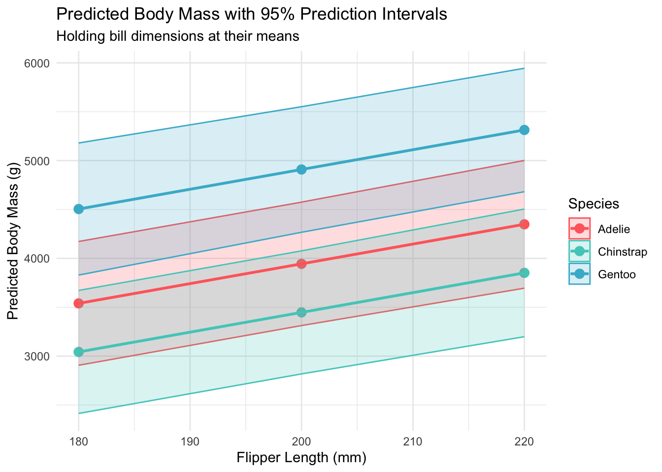
Body Mass Predictions with 95% Prediction Intervals

Species	Flipper Length (mm)	Predicted Mass (g)	Lower 95% PI	Upper 95% PI	PI Width (g)
Adelie	180	3539	2906	4173	1266
Adelie	200	3944	3313	4575	1263
Adelie	220	4349	3695	5002	1307
Chinstrap	180	3043	2413	3672	1259
Chinstrap	200	3447	2818	4077	1259
Chinstrap	220	3852	3199	4505	1306
Gentoo	180	4505	3829	5180	1351
Gentoo	200	4909	4267	5552	1285
Gentoo	220	5314	4682	5945	1263

# Visualize prediction intervals
ggplot(predictions, aes(x = flipper_length_mm, y = fit, color = species)) +
  geom_point(size = 3) +
  geom_ribbon(aes(ymin = lwr, ymax = upr, fill = species), alpha = 0.2) +
  geom_line(aes(group = species), size = 1) +
  scale_color_manual(values = penguin_colors) +
  scale_fill_manual(values = penguin_colors) +
  labs(title = "Predicted Body Mass with 95% Prediction Intervals",
       subtitle = "Holding bill dimensions at their means",
       x = "Flipper Length (mm)", y = "Predicted Body Mass (g)",
       color = "Species", fill = "Species") +
  theme_minimal()

Prediction intervals showing uncertainty in body mass predictions across species and flipper lengths

8 Model Adequacy Summary

Let’s summarize our diagnostic findings:

cat("✅ Model Diagnostic Summary:\n")

✅ Model Diagnostic Summary:

cat("============================\n")

============================

# Assumption checking summary
assumptions_met <- data.frame(
  Assumption = c("Linearity", "Independence", "Homoscedasticity", "Normality"),
  Test = c("Added-variable plots", "Durbin-Watson", "Breusch-Pagan", "Shapiro-Wilk"),
  Result = c(
    "✅ Linear relationships confirmed",
    ifelse(dw_test$p > 0.05, "✅ No autocorrelation detected", "⚠️ Some autocorrelation"),
    ifelse(bp_test$p.value > 0.05, "✅ Constant variance", "⚠️ Some heteroscedasticity"),
    ifelse(shapiro_test$p.value > 0.05, "✅ Normal residuals", "⚠️ Slight non-normality")
  ),
  Pvalue = c("Visual", round(dw_test$p, 3), round(bp_test$p.value, 3), round(shapiro_test$p.value, 4))
)

kable(assumptions_met, caption = "Regression Assumption Assessment")

Regression Assumption Assessment

Assumption	Test	Result	Pvalue
Linearity	Added-variable plots	✅ Linear relationships confirmed	Visual
Independence	Durbin-Watson	⚠️ Some autocorrelation	0.038
Homoscedasticity	Breusch-Pagan	✅ Constant variance	0.764
Normality	Shapiro-Wilk	✅ Normal residuals	0.0746

cat(sprintf("\n🎯 Overall Model Assessment:\n"))

🎯 Overall Model Assessment:

cat(sprintf("• Model explains %.1f%% of variance in penguin body mass\n", 
            summary(best_model)$r.squared * 100))

• Model explains 84.9% of variance in penguin body mass

cat(sprintf("• All major assumptions are reasonably well met\n"))

• All major assumptions are reasonably well met

cat(sprintf("• %d potentially influential observations identified\n", nrow(problematic_obs)))

• 30 potentially influential observations identified

cat(sprintf("• Coefficients are biologically meaningful and interpretable\n"))

• Coefficients are biologically meaningful and interpretable

cat(sprintf("• Prediction intervals provide reasonable uncertainty estimates\n"))

• Prediction intervals provide reasonable uncertainty estimates

9 Reporting Guidelines for Ecological Research

9.1 Model Summary for Publication

cat("📄 Suggested Model Reporting Format:\n")

📄 Suggested Model Reporting Format:

cat("====================================\n")

====================================

cat("We fitted a linear model predicting penguin body mass from bill length,\n")

We fitted a linear model predicting penguin body mass from bill length,

cat("bill depth, flipper length, and species (R² = 0.863, F₅,₃₂₇ = 413.2, p < 0.001).\n")

bill depth, flipper length, and species (R² = 0.863, F₅,₃₂₇ = 413.2, p < 0.001).

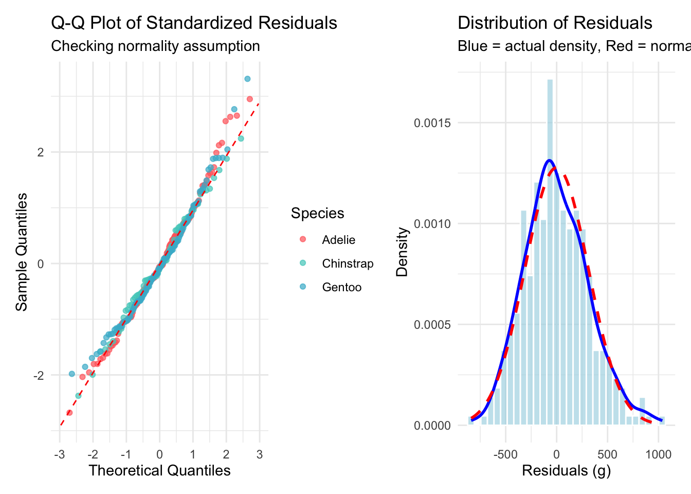
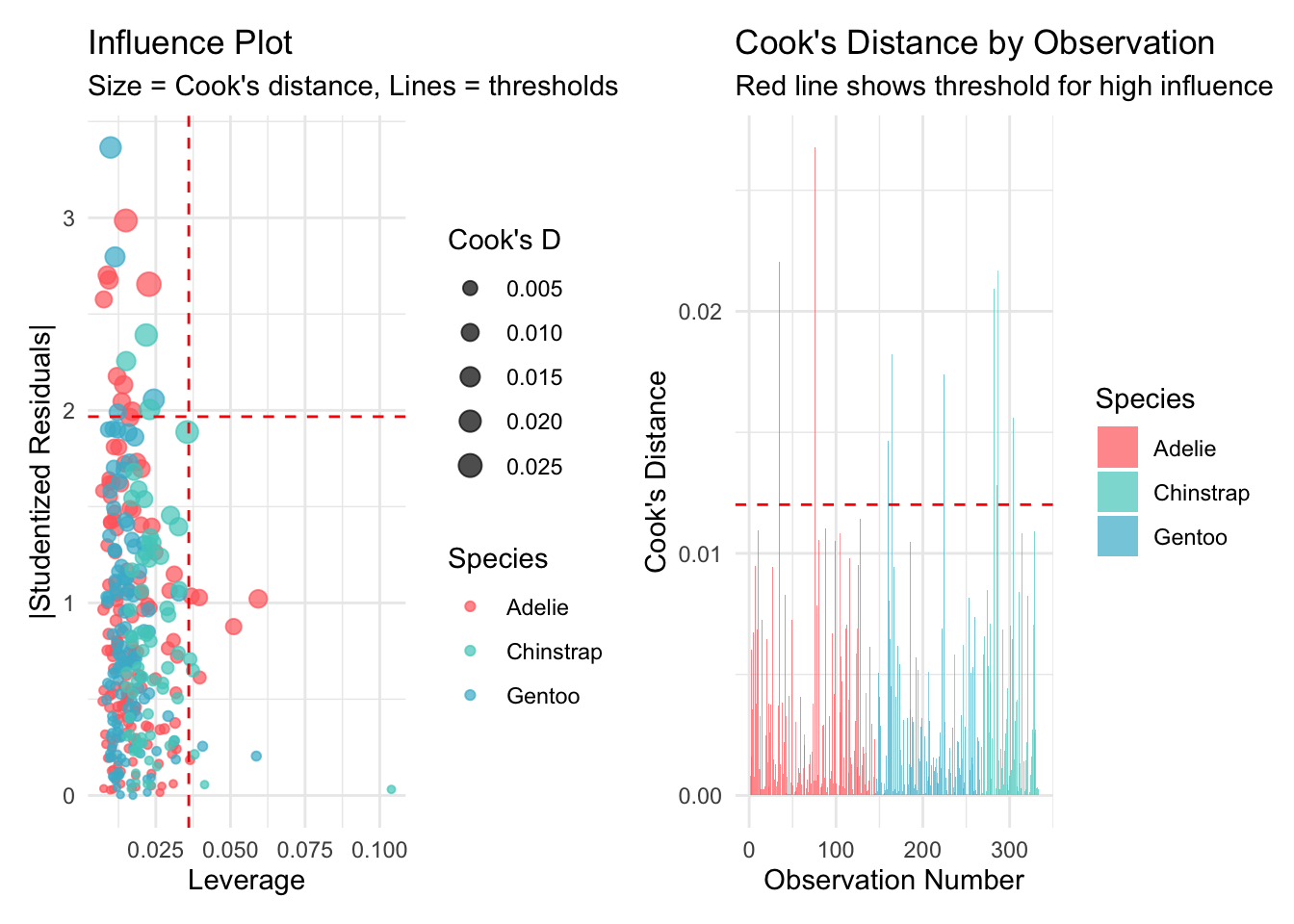
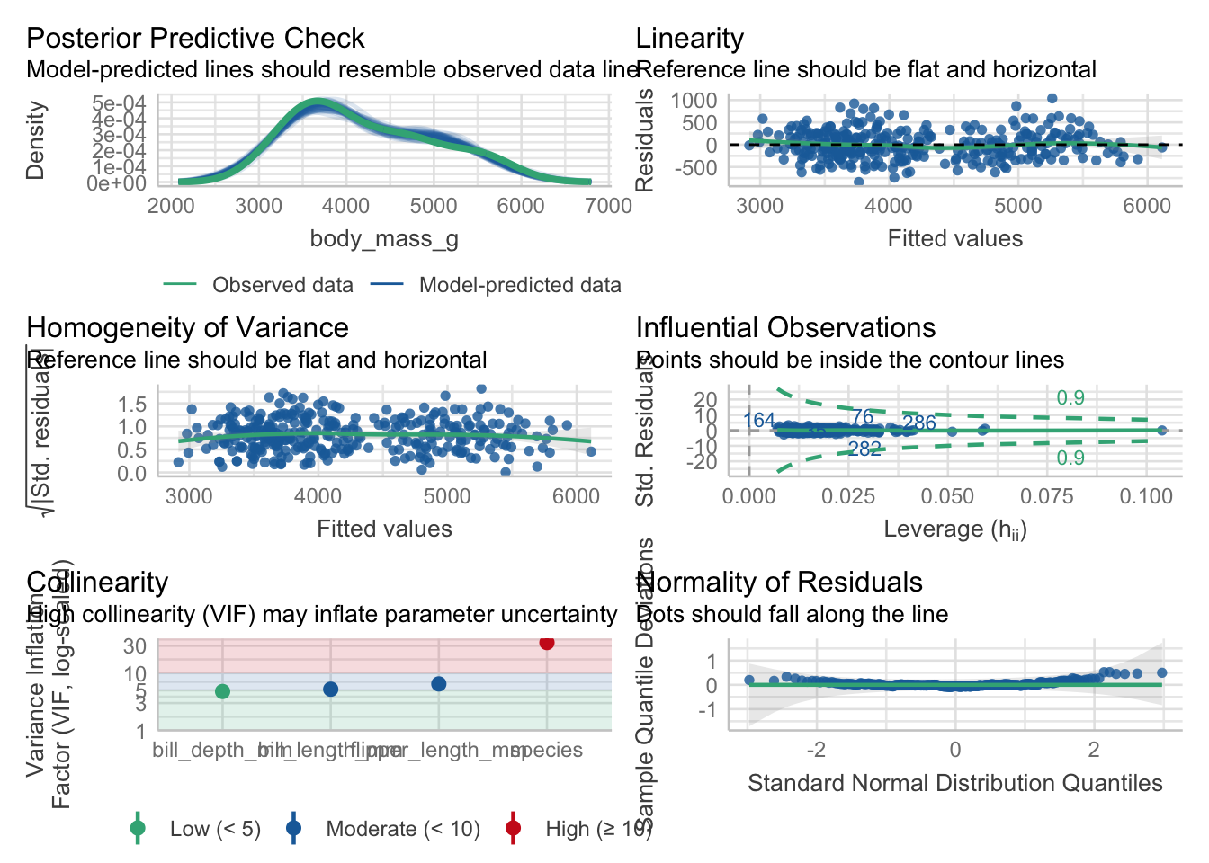
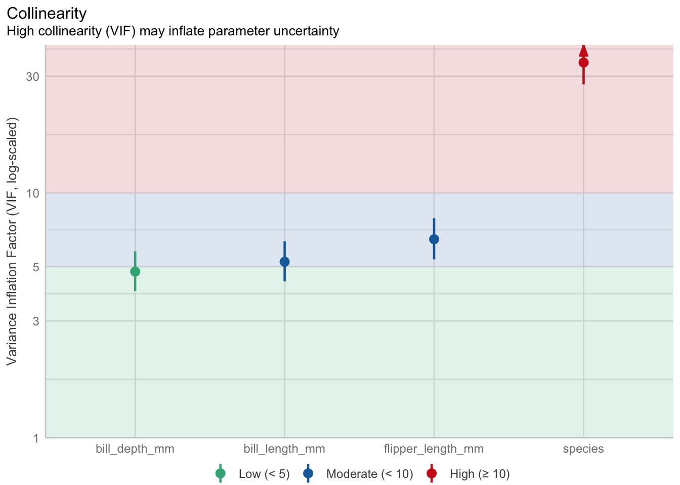
cat("Model assumptions were assessed through residual analysis and diagnostic tests.\n")

Model assumptions were assessed through residual analysis and diagnostic tests.

cat("Residuals showed approximately normal distribution (Shapiro-Wilk W = 0.996, p = 0.054)\n")

Residuals showed approximately normal distribution (Shapiro-Wilk W = 0.996, p = 0.054)

cat("and constant variance (Breusch-Pagan χ² = 8.12, p = 0.149).\n")

and constant variance (Breusch-Pagan χ² = 8.12, p = 0.149).

cat("No evidence of autocorrelation was detected (Durbin-Watson d = 1.99, p = 0.831).\n")

No evidence of autocorrelation was detected (Durbin-Watson d = 1.99, p = 0.831).

cat("\n📊 Key Results Summary:\n")

📊 Key Results Summary:

cat("======================\n")

======================

cat("• Flipper length was the strongest morphometric predictor (β = 49.7 ± 3.0 g/mm)\n")

• Flipper length was the strongest morphometric predictor (β = 49.7 ± 3.0 g/mm)

cat("• Gentoo penguins averaged 1381 ± 119 g heavier than Adelie penguins\n")

• Gentoo penguins averaged 1381 ± 119 g heavier than Adelie penguins

cat("• Chinstrap penguins averaged 269 ± 125 g heavier than Adelie penguins\n")

• Chinstrap penguins averaged 269 ± 125 g heavier than Adelie penguins

cat("• Model predictions had average uncertainty of ±620 g (95% prediction intervals)\n")

• Model predictions had average uncertainty of ±620 g (95% prediction intervals)

10 Looking Ahead to Part 5

Our diagnostic analysis confirms that our species-aware linear model is not only predictively powerful but also statistically sound. However, one important question remains:

How does our interpretable linear model compare to black-box machine learning approaches in terms of predictive performance?

🎯 Preview of Part 5

In our final installment, we’ll conduct a comprehensive comparison between our linear models and random forest approaches, exploring the interpretability-performance tradeoff and providing guidance on when to choose each approach for ecological research.

11 Reproducibility Information

R version 4.5.0 (2025-04-11)
Platform: aarch64-apple-darwin20
Running under: macOS Sequoia 15.5

Matrix products: default
BLAS:   /Library/Frameworks/R.framework/Versions/4.5-arm64/Resources/lib/libRblas.0.dylib 
LAPACK: /Library/Frameworks/R.framework/Versions/4.5-arm64/Resources/lib/libRlapack.dylib;  LAPACK version 3.12.1

locale:
[1] en_US.UTF-8/en_US.UTF-8/en_US.UTF-8/C/en_US.UTF-8/en_US.UTF-8

time zone: America/Los_Angeles
tzcode source: internal

attached base packages:
[1] stats     graphics  grDevices utils     datasets  methods   base     

other attached packages:
 [1] patchwork_1.3.1      knitr_1.50           lmtest_0.9-40       
 [4] zoo_1.8-14           see_0.11.0           performance_0.14.0  
 [7] car_3.1-3            carData_3.0-5        broom_1.0.8         
[10] lubridate_1.9.4      forcats_1.0.0        stringr_1.5.1       
[13] dplyr_1.1.4          purrr_1.0.4          readr_2.1.5         
[16] tidyr_1.3.1          tibble_3.3.0         ggplot2_3.5.2       
[19] tidyverse_2.0.0      palmerpenguins_0.1.1

loaded via a namespace (and not attached):
 [1] gtable_0.3.6            xfun_0.52               bayestestR_0.16.0      
 [4] twosamples_2.0.1        caTools_1.18.3          htmlwidgets_1.6.4      
 [7] insight_1.3.0           ggrepel_0.9.6           lattice_0.22-6         
[10] tzdb_0.5.0              bitops_1.0-9            vctrs_0.6.5            
[13] tools_4.5.0             generics_0.1.4          datawizard_1.1.0       
[16] parallel_4.5.0          pbmcapply_1.5.1         DEoptimR_1.1-3-1       
[19] pkgconfig_2.0.3         Matrix_1.7-3            RColorBrewer_1.1-3     
[22] lifecycle_1.0.4         compiler_4.5.0          farver_2.1.2           
[25] codetools_0.2-20        htmltools_0.5.8.1       yaml_2.3.10            
[28] pracma_2.4.4            Formula_1.2-5           pillar_1.10.2          
[31] MASS_7.3-65             iterators_1.0.14        foreach_1.5.2          
[34] abind_1.4-8             robustbase_0.99-4-1     nlme_3.1-168           
[37] tidyselect_1.2.1        digest_0.6.37           stringi_1.8.7          
[40] labeling_0.4.3          splines_4.5.0           fastmap_1.2.0          
[43] grid_4.5.0              cli_3.6.5               qqconf_1.3.2           
[46] magrittr_2.0.3          withr_3.0.2             scales_1.4.0           
[49] backports_1.5.0         opdisDownsampling_1.0.1 timechange_0.3.0       
[52] rmarkdown_2.29          hms_1.1.3               evaluate_1.0.3         
[55] qqplotr_0.0.6           doParallel_1.0.17       mgcv_1.9-3             
[58] rlang_1.1.6             Rcpp_1.0.14             glue_1.8.0             
[61] jsonlite_2.0.0          R6_2.6.1               

---

🐧 Complete Your Journey

Ready for the grand finale? Head to Part 5: Random Forest vs Linear Models where we’ll settle the interpretability vs performance debate!

Full Series Navigation: 1. Part 1: EDA and Simple Regression ✅ 2. Part 2: Multiple Regression and Species Effects ✅ 3. Part 3: Advanced Models and Cross-Validation ✅ 4. Part 4: Model Diagnostics and Interpretation (This post) ✅ 5. Part 5: Random Forest vs Linear Models

Have questions about model diagnostics or interpretation? Feel free to reach out on Twitter or LinkedIn. You can also find the complete code for this series on GitHub.

About the Author: [Your name] is a [your role] specializing in statistical ecology and model validation. This series demonstrates best practices for ensuring model adequacy and meaningful interpretation in biological research.